Consistency In College Basketball Statistics: Team-Based Trends and Analyses

The final in this three part exercise

Polygondwanaland

Now that we've explored the intersection of box score statistics and conference dynamics, we can shift the focus to individual teams within those conferences. Building on the use of coefficient of variation (CV) from Part One, we know that raw statistics tend to have higher variability than those adjusted for pace. Part Two showed that while consistency doesn't strongly correlate with winning, teams from conferences with tougher non-conference schedules often experience more volatility in their performance.

Although it's easy to make assumptions about a conference like the SWAC and the structural challenges that shape its schedule, greater granularity leads to stronger conclusions. By analyzing the matchups between Division I teams during the 2025 season, we can examine not only how individual teams perform, but also how their opponents perform against them.

Looking at the most and least volatile teams based on their average CV across all statistical categories, several trends begin to emerge.

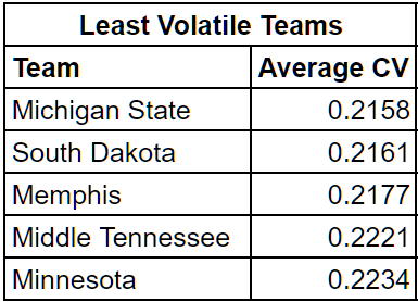
While looking at CV across statistical categories can feel unhelpful without context, it still offers a snapshot of the most consistent teams. Three of the most consistent teams come from high-major conferences. These teams often play weaker non-conference opponents relative to their conference schedule, which is reflected in the data. Minnesota, for example, had a soft non-conference slate but finished just 7–13 in the Big Ten, leaving little room for variability.

It's important to note that while most metrics account for strength of schedule, this consistency measure does not. Scoring 75 points against an elite defense and 75 against an average one would be weighted differently in traditional metrics, but here, they're treated identically.

Memphis played the fourth-toughest non-conference schedule in the country but are a big fish in the smaller AAC. In back-to-back seasons, they exceeded expectations in the non-conference before struggling in league play. Despite a few strong non-conference wins, they failed to dominate weaker AAC teams in the way you'd expect from a team of their caliber.

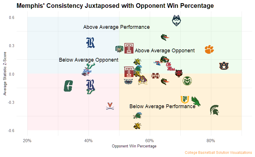
By comparing season-long averages to individual game performances, we can examine how Memphis' consistency varied depending on the opponent. They posted above-average performances against strong teams like UConn and Clemson, while games against the bottom of the conference—including USF, Charlotte, and Rice—saw them fall below their typical output. Their season-ending loss to Colorado State in the first round of the NCAA Tournament was a statistically average performance across the board.

Memphis played close games against both elite and mediocre opponents, which helps explain why they ranked as the third most consistent team in the country.

New Age Doom

Before diving into why the most consistent team performed the way it did, it's worth first looking at what defines teams that lack game-to-game consistency.

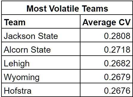
Notably, though not surprisingly, the two least consistent teams in the country are from the SWAC. This was a major focus in the second part of the series, where non-conference schedules filled with buy games led to significant disparities between games. All of the teams listed above are from low to mid-major conferences. Wyoming, which finished 12-20 overall and 5-15 in the Mountain West, is the team most adjacent to high-major status.

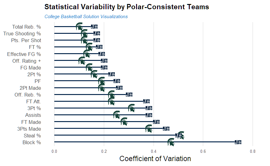
Contrasting Michigan State and Jackson State, the most and least consistent teams in the country, helps validate some earlier ideas. In part one, we identified block and steal percentage as the most volatile box score statistics. Fittingly, the one area where Michigan State is more volatile than Jackson State is in one of those same categories, reinforcing their status as inherently high-variance stats.

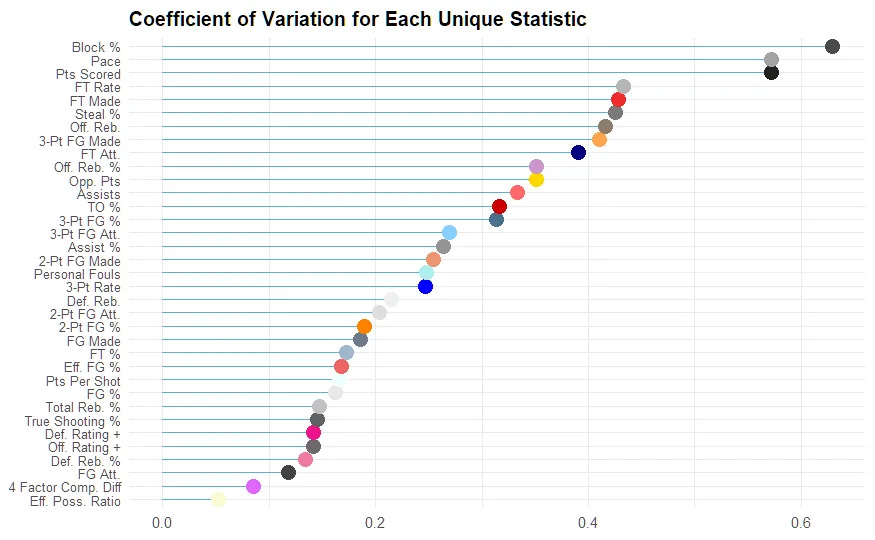
Another major discrepancy is free throws attempted, where Jackson State shows a much wider range than Michigan State. Two components of this—free throw rate and free throws made—rank as the fourth and fifth least consistent statistics, respectively. There is a clear explanation for why these statistics show large differences at a macro level, but understanding why these two teams are so far apart requires a closer look.

Some of this variation reflects broader contextual factors. Michigan State is coached by Tom Izzo, the second-longest tenured coach in Division I. His experience and system continuity likely contribute to the team's statistical consistency. Jackson State's volatility, on the other hand, is shaped by conference dynamics. They started the season 0–13 while playing a grueling non-conference slate of buy games to help fund their athletic department. The Tigers went on to finish 16–5, highlighting the dramatic difference between their early-season opponents and those faced in conference play.

If opponent quality explains much of this variability, it's worth comparing the statistics above with opponent output.

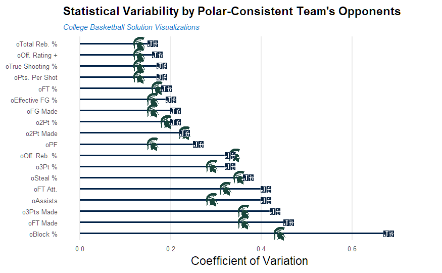
The gap for some of these statistics may not be what may have been expected, with opponent production seemingly more consistent than previously. In fact, the average difference of CV for the given team’s production is 0.08, compared to the same average for their opponent’s production being 0.0605. Thus, we can conclude that in this example of the most and least consistent teams, variance is more directly tied to the team’s performance, rather than their opponent’s performance. While this doesn’t remove the opponent from the equation of consistency, given an opponent can dictate play style, pace and plays defense at a varying level, the variance can be most directed internally.

Makeshift Tourniquet

At the end of the day, both Jackson State and Michigan State were good teams, relative to their conference. Jackson State fell by a mere four points in the SWAC championship game, despite their inconsistencies and 0-13 start. What matters, at the end of the day, is making the tournament. While Jackson State came just short of making the tournament, and while they could be tied to their overall consistency, if they were consistent in relevant statistical categories, then their other inconsistencies would be obsolete.

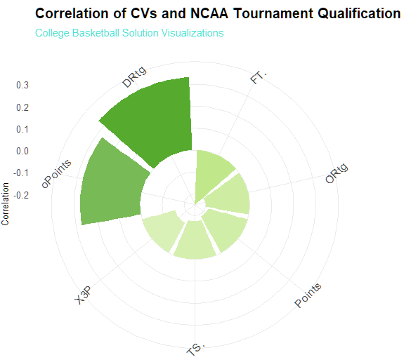
Defensive Rating and opponent points coefficient of variation show the strongest correlation with NCAA Tournament qualification. Since this correlation is positive, a higher CV is linked to qualification. Notably, inconsistent defensive performance is more strongly associated with making the tournament than consistent defense.

So, are defensive stats more effective with greater variance, while offensive stats benefit from consistency?

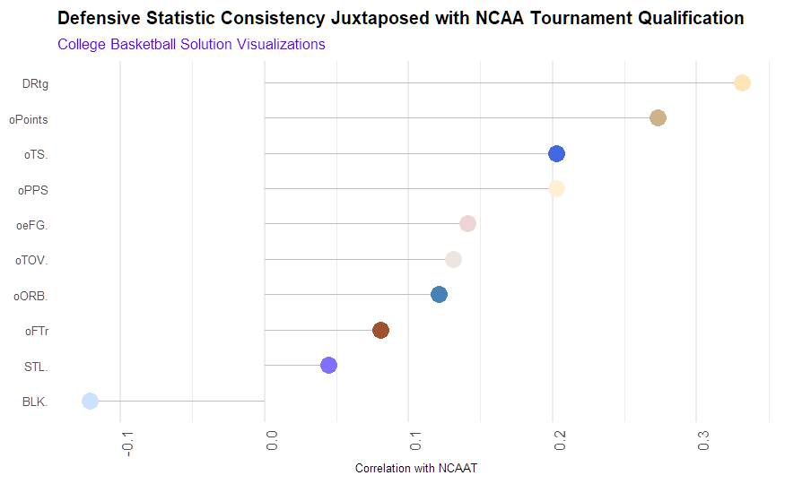
All but one of the selected defensive statistics show a correlation between higher CV and NCAA Tournament qualification. Block percentage, known for its high variability and impact on perception, is the only statistic that does not follow this trend.

How can a team’s opponent shooting variance be more favorable when inconsistent for tournament qualification? Each year, 70-75% of the NCAA Tournament field consists of high major teams. These teams often face lower-rated non-conference opponents and similarly ranked teams in conference play. While this pattern isn’t unique to high majors (as seen with the SWAC), it may help explain the defensive inconsistency.

Low and mid-major teams usually have contrasting schedules. Most teams that miss the tournament aren’t mediocre high majors but those from single-bid conferences who schedule opponents from lower leagues like the MAAC and NEC, then face other middling teams in conference play.

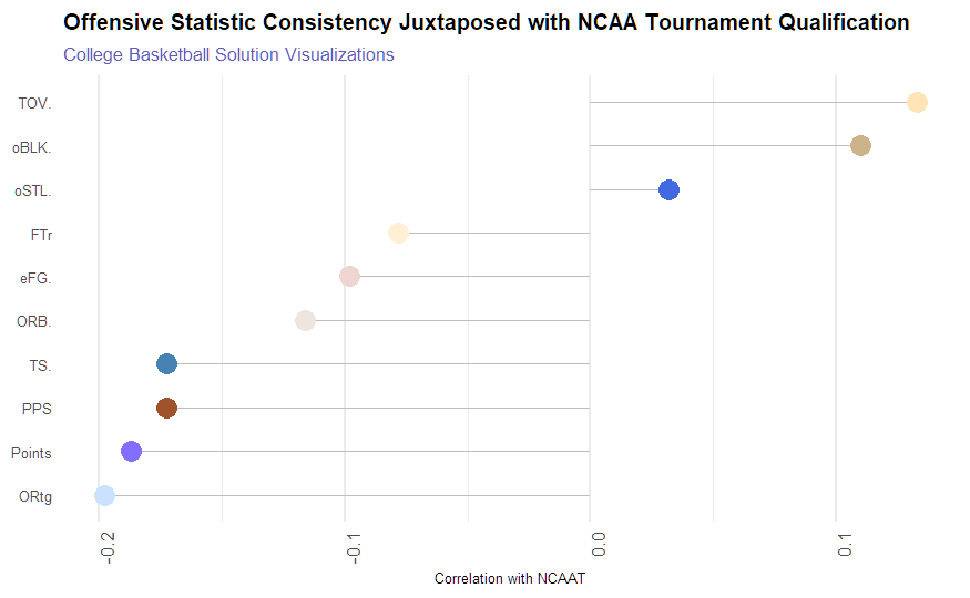
Many offensive statistics show the opposite pattern, except for turnover percentage and the opponent’s block and steal percentages. Block and steal percentages are generally considered random in terms of consistency. Turnover percentage suggests that teams with more variability in ball control are more likely to make the NCAA Tournament.

We’ve noted that tournament teams often face weaker opponents early in the season before tougher conference play. So why don’t we see the same inconsistency on offense?

Offense has fewer variables than defense. Teams can run similar plays and systems and take similar shots against most opponents. While offensive output may still vary, defenses are more likely to adjust their schemes to opponents than offenses are. Non-conference games against weaker teams may boost a tournament-bound team’s offensive stats, but this does not affect consistency.

Turnover percentage is therefore better explained by the opponent’s defensive system and pressure than by a team’s steady offensive performance.

Motionless Duties

Plotting Defensive and Offensive Rating consistency against each other shows that top teams like Gonzaga, Houston, Maryland, BYU, and national champion Florida fall into what we call the “Sweet Spot.”

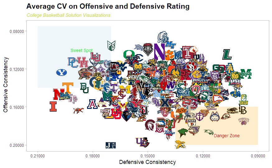
Teams with inconsistent offenses but steady defenses include Chicago State and Canisius, with Troy as one of the few tournament teams near this risky zone.

While this analysis offers some insights, the key takeaway is that without knowing the opponents, overall consistency means little. Making broad claims about many teams using both logic and statistics is difficult, especially without factors like opponent strength.

Consistency is just one layer in understanding what makes a team competitive. Seen through the right lens, it can help clarify some of the chaos. This three-part exercise didn’t yield definitive conclusions but revealed intriguing observations and subtle correlations in this puzzle we call college basketball.

-BM