Consistency In College Basketball Statistics: Macro-Level Trends in Box Scores

Part one of three

Marching Church

As February melts into March, making sense of the first five months of the college basketball season becomes crucial for analysts and fans alike. While averages offer a quick snapshot- highlighting strong shooting teams or elite rebounding units—they often oversimplify. Season-long averages can conceal the highs and lows. A team that shoots 38% from three might have reached that mark through a few hot shooting nights rather than consistent performance.

What matters in a single-elimination tournament isn’t what a team usually does—it’s what they might do on any given night. This kind of micro-level analysis is hard to pull off in the brief window between Selection Sunday and the Round of 64. Teams that built reputations on streaky performances make it difficult to project how they'll fare when the games truly count.

Take San Diego State. Viewed as a defensive juggernaut heading into their NCAA Tournament First Four matchup, they ranked among the top 15 in defensive efficiency. But in a blowout loss to North Carolina- their worst defensive showing of the season- the Aztecs’ reputation didn’t hold up. The graph below tracks their defensive rating across the year, revealing just how volatile that side of the ball really was.

Despite their strong overall defensive ranking, San Diego State allowed a defensive rating near 115 on five separate occasions before their tournament exit. Most of their best defensive efforts came early in the year, with a noticeable downward trend during conference play.

They weren’t alone. That kind of game-to-game volatility- the gap between a team’s best and worst showings- is more common than it might seem when looking only at season averages. To capture this hidden inconsistency, I analyzed the game logs of every Division I team, covering over 11,000 games, from both team’s perspective.

School of X

While this foundation may feel basic, it’s essential to understand the tools being used in the analysis. I relied on three key metrics for each team-stat combination:

• The mean summarizes the average performance for a given statistic across the sport. For instance, the average free throw percentage across Division I men's basketball last season was 71.9%.

• Standard deviation (SD) measures how much a team’s performance typically varies from game to game. It shows how far a single game might deviate from a team’s average. For free throw percentage, the SD is 0.12, meaning a typical team might shoot anywhere between 59.9% and 83.9% in a given game.

• The coefficient of variation (CV) accounts for differences in stat types—some are percentages (like free throw percentage), while others are whole numbers (like attempts). CV normalizes the data, allowing us to compare variability across all statistics. Free throw percentage, for example, falls around the 40th percentile in CV, meaning it’s a bit more stable than most other stats on a game-to-game basis. A higher CV indicates a statistic is more variable from game to game, while a lower CV points to greater consistency.

Highway Patrol

To measure consistency across the sport, I analyzed 94 different statistical variables drawn from team game logs. These stats fall into four broad categories:

• Game pace and its influence on scoring

• Shooting- including efficiency, frequency, and volume

• Rebounding, both offensive and defensive

• Ball control, encompassing both forced and committed turnovers

For each category, I also analyzed how well teams limited their opponents in those same areas. This matters on the micro level—when evaluating individual team defense—but it also plays a role on the macro level. Since every game is essentially mirrored (e.g., Florida vs. Houston is also Houston vs. Florida), opponent stats provide a second lens on the same event. Yet many of these mirrored stats are often overlooked in broader analyses of variability. By using the previously introduced coefficient of variation (CV), we can assess how consistent or erratic teams were across these categories from game to game.

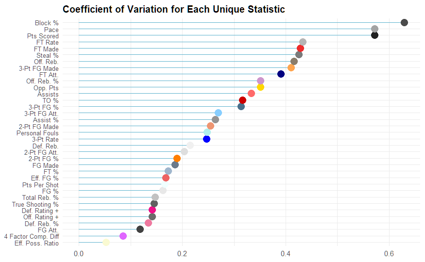
Let’s start with the stats that showed the least volatility. Among the most stable was Effective Possession Ratio (EPR), which is calculated by:

Scoring opportunities occur at a remarkably consistent rate across the sport. Similarly, pace- more reflective of game style than game results- remains relatively steady. Most Division I games fall between 63 and 73 possessions. In fact, per KenPom, only 11 teams during the 2025 season had an average pace outside of that range.

Juxtaposing this with the most volatile stats, these were largely defensive- most notably, blocks and steals.

On any given night, 95% of teams recorded somewhere between one and nine blocks. When the range is that small, a single block can shift perception dramatically. Steals and blocks also carry more scorekeeper subjectivity than, say, a made shot, which adds to their volatility.

The same idea applies to free throw rate, our fourth least consistent statistic- varied heavily based on officiating decisions. What a referee deems as a foul or non-foul introduces noise that doesn’t always reflect team behavior or defensive discipline.

Another highly inconsistent stats is Points Per Shot (PPS), which is calculated below:

The seemingly arbitrary 0.44 factor is used to adjust for the fact that not all free throws count as full possessions. Because games average just 63 to 73 possessions, a few highly efficient or inefficient possessions- especially early or late in halves- can significantly swing a team’s PPS. Composite metrics like PPS, which layer multiple components (free throws, shot attempts, field goal makes), tend to be more prone to volatility than simpler raw stats.

Unlucky for Some

The first statistic that might come to mind when thinking about inconsistency in college basketball is free throws. Fouls are called by different officials, in different environments, against different opponents—factors that seem ripe for unpredictability. Given this subjectivity, one might expect Free Throw Rate (FTR)—which measures how often a team gets to the line relative to its field goal attempts—to be the most variable statistics in the sport.

While there are some clear outliers- most notably a wild early-season matchup between UNC Wilmington and Georgia Southern that featured a staggering FTR of 1.180 (UNCW attempted 59 free throws in a 40-minute, 77-possession game)- the overall distribution of free throw rate is surprisingly narrow. The standard deviation for free throws attempted per game is just 5.9, meaning most teams fall within a relatively predictable range of about 12 attempts above or below the mean.

Part of this stability comes from the structural constraints of the game itself. With a limited number of possessions and foul limits that discourage excessive physicality, there’s only so much room for variation. Teams can’t draw (or commit) endless fouls without risking foul-outs or bonus situations that dramatically shift game flow.

Refereeing, while subjective, is also less chaotic than it might seem. Officials across the NCAA are trained under a common standard, which helps keep foul-calling relatively consistent from game to game. So while free throw rate remains one of the more variable stats compared to others, its variability is still more contained than one might expect at first glance.

Violent View

With a full overview of the variables— after removing any redundancy, clearer takeaways emerge.

One interesting pattern is the apparent link between the variability in shot volume and shooting efficiency. Teams that fluctuate widely in how many shots they take from a particular range also tend to fluctuate in how well they make them. There's no stabilizing trend: some teams take more two-point and three-point attempts and shoot them better, while others take more and shoot worse, just as some teams take fewer and perform better or worse.

Since this variability is greater than that of three-point rate alone, it suggests that teams largely stick to their preferred style of play: whether that means emphasizing shots inside or outside the arc, regardless of results.

Offensive and defensive rebounding show opposite ends of the variability spectrum, largely due to base frequency. A single offensive rebound has a much larger proportional impact on variation than a single defensive rebound. Offensive boards are both rarer and more dependent on team strategy. Some teams prioritize crashing the offensive glass, while others emphasize transition defense. On the other hand, defensive rebounding is not optional—every team must attempt to secure defensive boards, making it more consistent and less variable across games.

With a clearer picture of how box score statistics vary across the sport, we can now narrow the lens. Part two will explore how these patterns unfold within individual conferences—where factors like size, competitiveness, and team makeup influence how consistent (or random) the numbers really are.